Every integer greater than 1 is a product of primes in exactly one way, and this unit proves it, from the smallest divisor of a number to Euclid's lemma. It shows how the sieve of Eratosthenes finds every prime below a bound, why Euclid's argument gives endlessly many primes without a formula for them, how the exponents of a factorization answer questions about divisors, square roots, and factorials, and why recognizing a prime is a far easier task than factoring a number.
Sample unit: the complete text
Anyone can check in a minute that \(59 \times 509 = 30031\). Going the other way, from \(30031\) back to \(59\) and \(509\), takes a long time by hand, and for a product of two primes with a few hundred digits in all, no computer on Earth has managed it so far. That one-way quality of multiplication is the subject of this unit. It begins with the definition of a prime, proves that every integer is built from primes in exactly one way, shows how to find the primes below any bound, proves that they never run out, and ends with a question that still shapes computing: why deciding whether a number is prime is so much easier than taking it apart.
1 Primes and composites
Unit 2 introduced the notation \(a \mid b\), which says that \(a\) divides \(b\), that is, \(b = ac\) for some integer \(c\). An integer \(n > 1\) is called prime if its only positive divisors are \(1\) and \(n\) itself, and composite if it has a divisor \(d\) with \(1 < d < n\). The first primes are \(2, 3, 5, 7, 11, 13\), and the first composites are \(4, 6, 8, 9, 10, 12\). The number \(2\) is the only even prime, because every larger even number has the divisor \(2\).
The number \(1\) is neither prime nor composite, and this is a deliberate convention. If \(1\) counted as a prime, every integer would have infinitely many factorizations into primes, such as \(6 = 2 \cdot 3 = 1 \cdot 2 \cdot 3 = 1 \cdot 1 \cdot 2 \cdot 3\), and the theorem of Section 3, which says that the factorization is unique, would be false as stated. Keeping \(1\) out of the primes keeps the theorem clean.
The definition says what a prime is, and the first theorem says that every integer greater than \(1\) has one as a factor. To prove this, let \(n > 1\) and consider the set of divisors of \(n\) that are greater than \(1\). The set is not empty, because \(n\) belongs to it, so by the well-ordering principle of Unit 1, which says that every non-empty set of positive integers has a smallest element, it has a smallest element \(d\). This smallest divisor \(d\) must be a prime, for the following reason. If it were composite, it would have a divisor \(a\) with \(1 < a < d\), and since \(a \mid d\) and \(d \mid n\), the number \(a\) would be a divisor of \(n\) greater than \(1\) and smaller than \(d\), which contradicts the choice of \(d\).
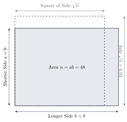
A second observation decides how much work it is to test a number. Suppose \(n\) is composite, so \(n = ab\) with \(1 < a \le b < n\). Then \(a \cdot a \le a \cdot b = n\), which gives \(a \le \sqrt{n}\), and the smallest prime factor \(p\) of \(a\), which is also a prime factor of \(n\) because \(p \mid a\) and \(a \mid n\), satisfies \(p \le a \le \sqrt{n}\). Figure 1 shows the idea as a rectangle. Its area is \(n\), and a rectangle cannot have both sides longer than the side of the square of the same area, so the shorter side is at most \(\sqrt{n}\).
Figure 1. A composite number \(n = ab\) drawn as a rectangle, here \(48 = 6 \times 8\), together with the square of the same area. The shorter side \(a\) never exceeds \(\sqrt{n}\), so the smallest prime factor of \(n\) is at most \(\sqrt{n}\), which for \(48\) means at most \(6\).
Trial division does two jobs at once, because if a prime divides \(n\), the quotient is a smaller number, the same procedure continues on it, and so the same method also factors \(n\) completely. The next example does both jobs by hand.
The second example answers a yes-or-no question and shows how the bound \(\sqrt{n}\) limits the work.
2 The sieve of Eratosthenes
Trial division tests one number at a time. To list all the primes below a bound \(N\), a different arrangement of the same work is far more efficient, and it is named after Eratosthenes of Cyrene (around 276 to 194 BC), the head of the library of Alexandria, who also measured the circumference of the Earth. The earliest surviving description is in the textbook Introduction to Arithmetic by Nicomachus of Gerasa (around AD 100), who attributes the method to Eratosthenes.
The sieve of Eratosthenes works as follows. Write down the integers from \(2\) to \(N\). The smallest of them, \(2\), is a prime; cross out all its multiples beyond itself. The smallest number still standing above \(2\) is \(3\), again a prime; cross out its multiples beyond itself, and continue in the same way. At every round the smallest number still standing that has not yet been used is a prime, because if it were composite it would be a multiple of some smaller number, and all those multiples have already been crossed out; its own multiples are crossed out next. Every number crossed out is a multiple of a smaller number and therefore composite, and every composite number is crossed out, because it is a multiple of its smallest prime factor, which is smaller than it. The numbers left standing at the end are exactly the primes up to \(N\).
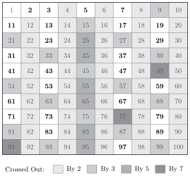
Two shortcuts follow from the observations of Section 1. When the multiples of a prime \(p\) are crossed out, the crossing can start at \(p^{2}\), because a smaller multiple \(kp\) with \(k < p\) has the factor \(k\), every prime factor of \(k\) is smaller than \(p\), and so \(kp\) was already crossed out in an earlier round. The same fact ends the sieve early. Once the current prime \(p\) satisfies \(p^{2} > N\), every composite number up to \(N\) has a prime factor below \(p\) and has already been crossed out, so the sieve may stop. For \(N = 100\) the sieve stops after the multiples of \(7\), since \(11^{2} = 121 > 100\).
Figure 2. The sieve of Eratosthenes on the numbers \(1\) to \(100\). Each composite number is shaded in the grey of the prime that crossed it out first, and the \(25\) numbers left standing in black are the primes below \(100\). The number \(1\) is left out of the sieve. Own computation.
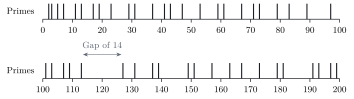
The sieve is also the simplest way to see how irregular the primes are. Figure 3 marks the \(46\) primes below \(200\) on a number line. Pairs that differ by \(2\), called twin primes, such as \(101\) and \(103\) or \(197\) and \(199\), sit next to stretches with no prime at all, such as the \(13\) composite numbers between \(113\) and \(127\). There is no visible rule for where the next prime falls, and no usable formula is known that produces the primes in order. What can be said is how many there are on average. The sieve gives \(25\) primes below \(100\), \(168\) below \(1000\), \(1229\) below \(10{,}000\), and \(78{,}498\) below one million, so the primes thin out, but slowly; Unit 8 says how many primes there are below a given size and why.
Figure 3. The primes below \(200\), found by the sieve, marked on a number line. The longest run without a prime below \(200\) is the gap of \(14\) between \(113\) and \(127\), while \(197\) and \(199\) differ by only \(2\). Own computation.
3 The fundamental theorem of arithmetic
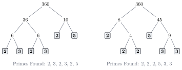
Figure 4 shows two ways of breaking \(360\) into factors. One starts with \(360 = 36 \times 10\), the other with \(360 = 8 \times 45\), and the two trees look different at every level, yet both end with the same primes: three \(2\)s, two \(3\)s, and one \(5\). Everyone who has factored numbers at school takes this for granted. It is a theorem, and its proof needs a fact about primes that is far from obvious.
Figure 4. Two factor trees of \(360\). The splits differ at every level, but both trees end with the primes \(2, 2, 2, 3, 3, 5\), as the fundamental theorem of arithmetic promises.
The fact is this: a prime that divides a product must divide one of the factors. For composite numbers the corresponding statement is false, since \(6\) divides \(4 \cdot 9 = 36\) and divides neither \(4\) nor \(9\). For primes it is true, and it goes back to Book VII of Euclid’s Elements.
The proof uses Bézout’s identity from Unit 2 in the form proved there: if \(d \mid ab\) and \(\gcd(d, a) = 1\), then \(d \mid b\). Suppose \(p \mid ab\) and \(p \nmid a\). The only positive divisors of \(p\) are \(1\) and \(p\), and \(p\) is not a divisor of \(a\), so \(\gcd(p, a) = 1\), and the result from Unit 2 gives \(p \mid b\). The statement for \(k\) factors follows by induction on \(k\), since \(p \mid a_1 (a_2 \cdots a_k)\) means that \(p\) divides \(a_1\) or divides the product of the remaining \(k - 1\) factors, and in the second case the statement for \(k - 1\) factors, already proved, names one of them.
With the lemma in hand, the theorem that gives the unit its title can be stated and proved. It appears in Euclid’s Elements only in special cases; the first complete statement and proof are in the book Disquisitiones Arithmeticae (1801) of Carl Friedrich Gauss (1777-1855).
The theorem has two halves, existence and uniqueness, and they are proved by different means. Existence uses strong induction, which Unit 1 introduced, and uniqueness uses Euclid’s lemma.
The argument deserves a second look at the one place where it could fail. In the uniqueness half, \(p_1 \mid q_1 q_2 \cdots q_m\) had to force \(p_1\) to divide a single \(q_j\). That step is Euclid’s lemma, which rests on Bézout’s identity, which rests on division with remainder, and the whole theorem hangs on that chain. The excursion below shows a number system in which the chain breaks.
Because the factors can be collected, the theorem has a standard shorthand. Grouping equal primes and ordering them by size gives the canonical factorization.
The exponent notation obeys one rule that is used constantly. For positive integers \(a\) and \(b\), the factorization of \(ab\) is the product of the factorizations of \(a\) and \(b\), and by uniqueness it is the only factorization of \(ab\), so
\begin{equation}
v_p(ab) = v_p(a) + v_p(b) \qquad \text{for every prime } p . \label{eq:vp}
\end{equation}
4 Reading the factorization
Once \(n\) is written in canonical form, questions about its divisors become questions about exponents. The link is that an integer \(d > 0\) divides \(n\) if and only if \(v_p(d) \le v_p(n)\) for every prime \(p\). In one direction, if \(d \mid n\), then \(n = dc\) and Equation \eqref{eq:vp} gives \(v_p(n) = v_p(d) + v_p(c) \ge v_p(d)\). In the other direction, if all exponents of \(d\) are at most those of \(n\), then \(n/d\) is the integer with exponents \(v_p(n) - v_p(d)\), so \(d\) divides \(n\). So the divisors of \(n = p_1^{e_1} \cdots p_k^{e_k}\) are exactly the numbers \(p_1^{f_1} \cdots p_k^{f_k}\) with \(0 \le f_i \le e_i\). For example, the divisor \(18 = 2^{1} \cdot 3^{2} \cdot 5^{0}\) of \(360 = 2^{3} \cdot 3^{2} \cdot 5\) chooses the exponents \(1\), \(2\), and \(0\). For each prime there are \(e_i + 1\) choices of exponent, and the choices are independent, which counts the divisors at once.
4.1 Greatest common divisor and least common multiple
A common divisor \(d\) of \(a\) and \(b\) must satisfy \(v_p(d) \le v_p(a)\) and \(v_p(d) \le v_p(b)\) for every \(p\), and the largest such \(d\) takes the smaller of the two exponents at each prime. A common multiple must have exponents at least as large as both, and the smallest takes the larger of the two.
For two numbers of modest size, the exponent rule and Euclid’s algorithm cost about the same. For two numbers of three hundred digits the difference is enormous: Euclid’s algorithm finishes in at most \(1500\) steps by Lamé’s bound of Unit 2, which allows five steps for every decimal digit, whereas nobody can factor the numbers. The exponent rule is a way of understanding the gcd, and Euclid’s algorithm is the way of computing it.
4.2 Square roots
Unit 1 proved that \(\sqrt{2}\) is irrational by an argument about even and odd numbers. Unique factorization turns that argument into a rule for every integer. Suppose \(\sqrt{n} = a/b\) with positive integers \(a\) and \(b\). Squaring and clearing the denominator gives \(n b^{2} = a^{2}\), and Equation \eqref{eq:vp} applied to both sides gives, for every prime \(p\),
\[
v_p(n) + 2\,v_p(b) = 2\,v_p(a) .
\]
The right side is even and \(2 v_p(b)\) is even, so \(v_p(n)\) is even for every prime \(p\), which means that \(n\) is the square of the integer \(\prod p^{v_p(n)/2}\), the product over the primes dividing \(n\) of each prime raised to half its exponent (the product sign \(\prod\) is the one Unit 1 introduced). In words, the square root of a positive integer is either an integer or irrational, and nothing in between. For example, \(12 = 2^{2} \cdot 3\) has \(v_3(12) = 1\), which is odd, so \(\sqrt{12}\) is irrational, and the same reasoning with cube roots and \(3 v_p(b)\) shows that \(\sqrt[3]{n}\) is irrational unless \(n\) is a cube.
4.3 The exponent of a prime in a factorial
How many times does \(p\) divide the factorial \(n! = 1 \cdot 2 \cdot 3 \cdots n\)? Among the factors \(1, 2, \ldots, n\), every \(p\)-th one is a multiple of \(p\), so there are \(\lfloor n/p \rfloor\) of them, where \(\lfloor x \rfloor\) is the floor of \(x\), the largest integer not exceeding \(x\) (Unit 1). That is not the whole count, because the multiples of \(p^{2}\) contribute a second factor \(p\) each, the multiples of \(p^{3}\) a third, and so on. Adrien-Marie Legendre (1752-1833) wrote the resulting formula in his book Essai sur la théorie des nombres (second edition, 1808).
Beyond this unit, Legendre’s formula serves in a different role, as a tool for estimating how many primes there are below a given size. For now it is the first example of a principle that runs through the whole subject: a statement about a huge number, here \(100!\), can often be settled by counting its prime factors instead of computing it.
5 Euclid’s theorem
The sieve produces as many primes as patience allows, but no amount of sieving shows that the supply never ends. The proof that it does not is Proposition 20 of Book IX of Euclid’s Elements (around 300 BC), and it is one of the oldest proofs in mathematics that is still taught in its original form.
Euclid (active around 300 BC) stated the result as “prime numbers are more than any assigned multitude of prime numbers” and proved it for a list of three primes, which is the general case in the notation of his time. His argument is not a proof by contradiction, although it is often retold as one. It is a direct construction: given any primes, it points at a number whose prime factors are new. The construction does not say that \(N\) itself is prime, and usually it is not.
The same idea reaches a little further. Every odd prime leaves the remainder \(1\) or \(3\) on division by \(4\), because the remainders \(0\) and \(2\) belong to even numbers, and the list \(3, 7, 11, 19, 23, 31, \ldots\) of primes with remainder \(3\) is also endless.
The primes with remainder \(1\), namely \(5, 13, 17, 29, \ldots\), are also infinite in number, but the trick with \(N\) does not reach them, and a different idea is needed, which is beyond this unit. The general statement, that every progression \(a, a + q, a + 2q, \ldots\) with \(\gcd(a, q) = 1\) contains infinitely many primes (the condition is needed, since otherwise every term is divisible by \(\gcd(a, q)\)), is Dirichlet’s theorem on primes in arithmetic progressions, proved by Peter Gustav Lejeune Dirichlet (1805-1859) in 1837 with tools from analysis that lie far beyond this masterclass.
6 Recognizing primes and factoring them
Two questions look alike and are not. The first asks whether a given \(n\) is prime; the second asks for its factors. Trial division answers both, but at a price of up to about \(\sqrt{n}\) divisions, and \(\sqrt{n}\) grows by a factor of \(10\) for every two digits added to \(n\). A \(50\)-digit number needs \(10^{25}\) divisions, which no computer will finish; at a billion divisions a second, that would take about \(300\) million years. This section shows that the first question has a fast answer, that the second does not, as far as anyone knows, and that the gap between the two is what modern cryptography is built on.
6.1 Mersenne primes and the Lucas-Lehmer test
Nearly every record prime of the computer age has the form \(2^{p} - 1\); such numbers are named Mersenne numbers after Marin Mersenne (1588-1648), a French monk who corresponded with most of the mathematicians of his time and published a list of the exponents he believed gave primes. If \(2^{n} - 1\) is prime, then \(n\) must be prime; Unit 6 proves this with an algebraic identity. The converse, that \(2^{p} - 1\) is prime for every prime \(p\), is false, as the example \(2^{11} - 1 = 2047 = 23 \times 89\) shows. The reason these numbers are the record holders is that a prime of this special form can be recognized far faster than a general number of the same size.
For \(p = 7\) and \(M_7 = 127\) the remainders are \(s_0 = 4\), \(s_1 = 14\), \(s_2 = 194 - 127 = 67\), \(s_3 = 67^{2} - 2 = 4487 \equiv 42\), \(s_4 = 42^{2} - 2 = 1762 \equiv 111\), and \(s_5 = 111^{2} - 2 = 12319 = 97 \cdot 127 \equiv 0\), so \(127\) is prime. Five squarings replaced the trial divisions. For \(p = 136{,}279{,}841\) the test needs about \(136\) million squarings of numbers with \(41\) million digits, which is a large computation and a possible one, whereas trial division of a number of that size is not possible in the lifetime of the universe. Table 1 lists a selection of the \(52\) Mersenne primes known in October 2024, with the largest known prime, \(2^{136279841} - 1\), at the end.
Exponent \(p\)
Digits
Year
Found By
Method
17
6
1588
P. Cataldi
trial division
31
10
1772
L. Euler
trial division
127
39
1876
É. Lucas
Lucas’s test, by hand
521
157
1952
R. Robinson
Lucas-Lehmer, SWAC
11,213
3376
1963
D. Gillies
Lucas-Lehmer, ILLIAC II
1,398,269
420,921
1996
J. Armengaud, GIMPS
Lucas-Lehmer, home PC
82,589,933
24,862,048
2018
P. Laroche, GIMPS
Lucas-Lehmer, home PC
136,279,841
41,024,320
2024
L. Durant, GIMPS
probable-prime test, GPUs
Table 1. Eight of the \(52\) known Mersenne primes \(2^{p} - 1\), with the number of decimal digits of each, from the first proved by trial division to the largest known prime, found on 12 October 2024. Data from the GIMPS list of known Mersenne primes, mersenne.org.
6.2 Recognizing against factoring
A Mersenne number is a special case. For a general \(n\), the fast tests in use rest on Fermat’s little theorem, which Unit 5 proves: for a prime \(p\) and an integer \(a\) not divisible by \(p\), the power \(a^{p-1}\) leaves the remainder \(1\) on division by \(p\). A number that fails this for some \(a\) is certainly composite, and the test says so without producing a factor. Unit 5 shows how the idea is refined into the tests with which software finds primes of \(300\) digits, the building blocks of the RSA keys that encrypt internet traffic, which Unit 5 also explains, in a fraction of a second each.
Factoring has no such shortcut. The best known methods are far better than trial division, but they still take time that grows faster than any power of the number of digits. The record for a number with two prime factors of equal size is RSA-250, a number of \(250\) decimal digits (829 binary digits), factored in February 2020 by a team of French and American researchers. The computation took about \(2700\) core-years, which means that a single processor core would have needed \(2700\) years, and the work was spread over thousands of cores for several months. For comparison, the primality of a \(250\)-digit number is decided in milliseconds.
The scale of the two tasks is best described with the number of digits of \(n\), which Unit 1 wrote as \(\lfloor \log_{10} n \rfloor + 1\). An algorithm runs in polynomial time if the number of steps it needs is bounded by a fixed power of the number of digits, such as the square or the cube. Adding, multiplying, and Euclid’s algorithm are all polynomial. Trial division is not, since \(\sqrt{n}\) is about \(10^{D/2}\) for a \(D\)-digit number, which grows faster than any power of \(D\). The fast primality tests based on Fermat’s theorem are polynomial, but for decades every one of them either used random choices or relied on an unproved conjecture. Whether primality could be decided in polynomial time with no randomness and no conjecture was an open question until 2002, and it is the subject of the research spotlight below.
Figure 5. Lehmer sieves at the Computer History Museum in Mountain View, California. Each loop or wheel in such a machine stands for one small modulus and carries holes at the remainders that are allowed; the machine advances all of them in step and signals when a hole of every one lines up. Credit: Carlo Nardone, Wikimedia Commons, CC BY-SA 2.0.
This is one of 16 units
Participants also get the quiz, the further reading, and the final exam.